Hi bonnie, I changed the chunk option above to make the default behaviour echo = TRUE. It makes the code and output appear in your document.
Summary
Obesity is a growing health and financial burden across the world, and as such, it is becoming increasingly important to identify, and reduce or eliminate, risk factors for obesity. Research from the early 2000s suggests that low SES in childhood is a major predictor of obesity and insulin resistance in adulthood. This finding is consistent with life-history theory, which predicts that experience of conditions typical of low SES-environments in childhood will shape development such that the child learns how best to survive in harsh and unpredictable environments. That is, an individual may learn to eat as much as they can and whenever they can, if they grew up in a low SES-environment where food was unreliable or frequently unavailable.
In line with these early findings and life-history theory, Hill and colleagues (2016) examined the relationship between childhood socioeconomic status (SES) and eating in the absence of energy need. In a series of studies, researchers measured or manipulated (by asking participants to fast for 5 hours) each participant’s current energy need, quantified as length of time since last meal, current level of hunger and/or blood glucose levels. Researchers then provided participants with the opportunity to eat snack foods. Participants reported their childhood and current SES.
Participants who grew up in high SES environments regulated their food intake according to their energy need. These participants ate more when their need was high than they did when their need was low. Conversely, participants who grew up in low SES consumed comparably large amounts of food when their energy need was both high and low. The researchers concluded that childhood SES may influence how an individual responds to internal, physiological cues in adulthood.
Plan
There are 3 studies reported in this paper. For each study, the goal is to reproduce the …
- demographic descriptives (reported in Participants)
- figures (column graphs reporting total calories as a function of SES and energy need/condition/glucose)
- tables of descriptive statistics (M, SD, Range)
demographics
For each study the authors report…
- how many students participated
- mean, SD, range age
They only included those with BMI < 30 and excluded those with food allergies or diabetes
Study 1
read in the data
Use the here() function to tell R where to find your data. And use clean_names() from janitor to make the variable names easier to work with.
s1 <- read_csv(here("research_data", "eating_correlational.csv"))
  cleans1 <- clean_names(s1)
Use glimpse() to familiarise yourself with what is in the file and find the demographic variables.
glimpse(cleans1)
Rows: 31
Columns: 25
$ p_id                        <dbl> 101, 102, 103, 104, 105, 106, 10…
$ sex                         <dbl> 2, 2, 2, 2, 2, 2, 2, 2, 2, 2, 2,…
$ age                         <dbl> 21, 19, 22, 21, 19, 20, 22, 18, …
$ weight_1                    <dbl> 140, 138, 145, 160, 102, 110, 18…
$ hungercurr                  <dbl> 6, 2, 5, 2, 6, 4, 5, 2, 4, 4, 4,…
$ hunger_recode               <dbl> 2, 6, 3, 6, 2, 4, 3, 6, 4, 4, 4,…
$ lastate_1                   <dbl> 0, 2, 1, 3, 2, NA, 1, 10, 9, 10,…
$ z_hunger_recode             <dbl> -1.7342012, 1.3823343, -0.955067…
$ zlastate_1                  <dbl> -1.03257585, -0.51179846, -0.772…
$ z_last_ate_hunger_composite <dbl> -1.38338854, 0.43526792, -0.8636…
$ p_delicious                 <dbl> 5, 5, 5, 4, 6, 5, 6, 7, 6, 5, 7,…
$ c_delicious                 <dbl> 7, 6, 6, 5, 5, 6, 5, 7, 7, 6, 4,…
$ familmoney                  <dbl> 6, 6, 7, 6, 6, 5, 7, 2, 7, 6, 7,…
$ neighborho                  <dbl> 6, 7, 7, 3, 4, 3, 6, 2, 5, 4, 7,…
$ wealthcomp                  <dbl> 6, 5, 7, 2, 4, 4, 6, 4, 6, 3, 6,…
$ childhood_ses_composite     <dbl> 6.000000, 6.000000, 7.000000, 3.…
$ weight_cookies_pre          <dbl> 59, 62, 60, 59, 59, 60, 61, 58, …
$ weight_pretzels_pre         <dbl> 30, 30, 30, 29, 30, 30, 30, 30, …
$ weight_cookies_post         <dbl> 45, 4, 45, 39, 30, 27, 54, 3, 3,…
$ weight_pretzels_post        <dbl> 22, 8, 22, 16, 26, 15, 28, 21, 2…
$ grams_pretzels_eaten        <dbl> 8, 22, 8, 13, 4, 15, 2, 9, 10, 9…
$ grams_cookies_eaten         <dbl> 14, 58, 15, 20, 29, 33, 7, 55, 5…
$ pretzel_calories_eaten      <dbl> 30.760, 84.590, 30.760, 49.985, …
$ cookie_calories_eaten       <dbl> 70, 290, 75, 100, 145, 165, 35, …
$ total_calories_eaten        <dbl> 100.760, 374.590, 105.760, 149.9…
count the participants
Use the count function to count how many participants there were. Are those that were excluded due to BMI or allergies/diabetes included in the dataset??
count(cleans1, "p_id")
# A tibble: 1 x 2
  `"p_id"`     n
* <chr>    <int>
1 p_id        31
31 participants. Participants excluded due to BMI/allergies/diabetes not included in dataset.
summarise age
Use the summarise function to get the mean, sd, min, and max age
cleans1 %>%
  summarise(meanage = mean(age, na.rm = TRUE),
          sdage = sd(age, na.rm = TRUE),
          minage = min(age, na.rm = TRUE),
          maxage = max(age, na.rm = TRUE))
# A tibble: 1 x 4
  meanage sdage minage maxage
    <dbl> <dbl>  <dbl>  <dbl>
1    19.2  1.26     18     22
Study 2
As for study 1, read in the data for Study 2, use count() to see how many participants there were, and summarise to get M, SD, min, and max age.
s2 <- read_csv(here("research_data", "eating_drink.csv"))
  cleans2 <- clean_names(s2)
count the participants
count(cleans2, "p_id")
# A tibble: 1 x 2
  `"p_id"`     n
* <chr>    <int>
1 p_id        60
summarise age
cleans2 %>%
  summarise(meanage = mean(age, na.rm = TRUE),
          sdage = sd(age, na.rm = TRUE),
          minage = min(age, na.rm = TRUE),
          maxage = max(age, na.rm = TRUE))
# A tibble: 1 x 4
  meanage sdage minage maxage
    <dbl> <dbl>  <dbl>  <dbl>
1    19.3  1.52     18     24
count condition assignment
Which variable contains info about the condition participant were assigned to? Use tabyl to count how many were assigned to each condition.
dummy1_water_sprite & dummy2_sprite_water
cleans2 %>%
  tabyl(dummy1_water_sprite)
 dummy1_water_sprite  n   percent
                   0 29 0.4833333
                   1 31 0.5166667
cleans2 <- cleans2 %>%
mutate(condition = case_when(dummy1_water_sprite == 1 ~ "water",
dummy1_water_sprite == 0 ~ "sprite")) %>%
relocate(condition, .before = "gender")
names(cleans2)
 [1] "participant_id"      "dummy1_water_sprite" "dummy2_sprite_water"
 [4] "condition"           "gender"              "age"
 [7] "weight_1"            "hrs_no_eat_1"        "hunglvl"
[10] "delicious_taste"     "currnt_ses"          "child_ses"
[13] "fam_money"           "wlthy_ngbr"          "wlth_kids"
[16] "hrs_eat_check"       "foodweigh1"          "foodweigh2"
[19] "food_eaten"          "calories_eaten"      "finish_drink"
[22] "drink_drank_oz"      "childhood_ses_mean"
Sprite = 31; Water = 29
Study 3
Read the data and then use the count function to count how many participants there were in total and the tabyl function to count how many were men and women. Use summarise to get the mean, sd, min, and max age.
s3 <- read_csv(here("research_data", "eating_glucose.csv"))
  cleans3 <- clean_names(s3)
count the participants
count(cleans3, "p_id")
# A tibble: 1 x 2
  `"p_id"`     n
* <chr>    <int>
1 p_id        83
summarise age
cleans3 %>%
  summarise(meanage = mean(age, na.rm = TRUE),
          sdage = sd(age, na.rm = TRUE),
          minage = min(age, na.rm = TRUE),
          maxage = max(age, na.rm = TRUE))
# A tibble: 1 x 4
  meanage sdage minage maxage
    <dbl> <dbl>  <dbl>  <dbl>
1    20.1  1.96     18     27
count male/female
cleans3 %>%
  tabyl(gender)
 gender  n  percent
      1 21 0.253012
      2 62 0.746988
Tables
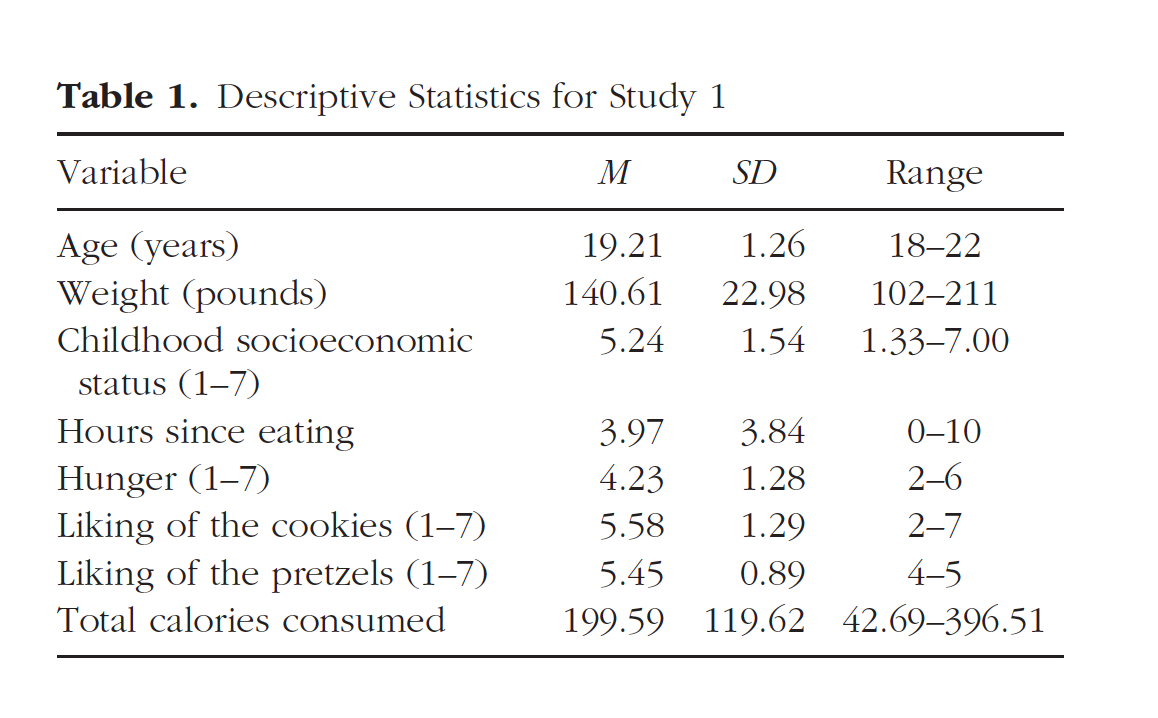
Study 1
The goal is to reproduce the values and formatting of this table.
knitr::include_graphics(here::here("img","paper1_table1.png"))
Using arsenal
table_one <- tableby(~ age + weight_1 + childhood_ses_composite + lastate_1 + hungercurr + c_delicious + p_delicious + total_calories_eaten,
                     data = cleans1)

my_labels <- list(
  age = "Age (years)",
  weight_1 = "Weight (pounds)",
  childhood_ses_composite = "Childhood socioeconomic status (1-7)",
  lastate_1 = "Hours since eating",
  hungercurr = "Hunger (1-7)",
  c_delicious = "Liking of the cookies (1-7)",
  p_delicious = "Liking of the pretzels (1-7)",
  total_calories_eaten = "Total calories consumed"
)
summary(table_one, labelTranslations = my_labels,
        title = "Table 1. Descriptive Statistics for Study 1")
| Overall (N=31) | |
|---|---|
| Age (years) | |
| N-Miss | 3 |
| Mean (SD) | 19.214 (1.258) |
| Range | 18.000 - 22.000 |
| Weight (pounds) | |
| Mean (SD) | 140.613 (22.976) |
| Range | 102.000 - 215.000 |
| Childhood socioeconomic status (1-7) | |
| Mean (SD) | 5.247 (1.540) |
| Range | 1.333 - 7.000 |
| Hours since eating | |
| N-Miss | 2 |
| Mean (SD) | 3.966 (3.840) |
| Range | 0.000 - 10.000 |
| Hunger (1-7) | |
| Mean (SD) | 3.774 (1.283) |
| Range | 2.000 - 6.000 |
| Liking of the cookies (1-7) | |
| Mean (SD) | 5.581 (1.285) |
| Range | 2.000 - 7.000 |
| Liking of the pretzels (1-7) | |
| Mean (SD) | 5.452 (0.888) |
| Range | 4.000 - 7.000 |
| Total calories consumed | |
| Mean (SD) | 199.588 (119.526) |
| Range | 42.690 - 396.505 |
- checking missing values
https://cran.r-project.org/web/packages/naniar/vignettes/getting-started-w-naniar.html
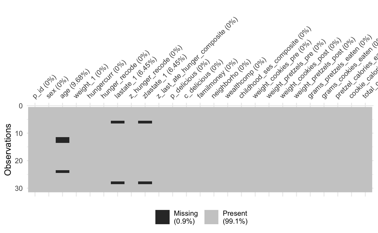
cleans1_nona <- cleans1 %>%
  na.omit()

cleans1_agena <- cleans1 %>%
  drop_na(age)
table_two <- tableby (~ age + weight_1 + childhood_ses_composite + lastate_1 + hungercurr + c_delicious + p_delicious + total_calories_eaten, data = cleans1)

summary(table_two,
        labelTranslations = my_labels,
        title = "Table 1. Descriptive Statistics for Study 1")
Table: (\#tab:unnamed-chunk-20)Table 1. Descriptive Statistics for Study 1
| | Overall (N=31) |
|:----------------------------------------|:-----------------:|
|**Age (years)** | |
| N-Miss | 3 |
| Mean (SD) | 19.214 (1.258) |
| Range | 18.000 - 22.000 |
|**Weight (pounds)** | |
| Mean (SD) | 140.613 (22.976) |
| Range | 102.000 - 215.000 |
|**Childhood socioeconomic status (1-7)** | |
| Mean (SD) | 5.247 (1.540) |
| Range | 1.333 - 7.000 |
|**Hours since eating** | |
| N-Miss | 2 |
| Mean (SD) | 3.966 (3.840) |
| Range | 0.000 - 10.000 |
|**Hunger (1-7)** | |
| Mean (SD) | 3.774 (1.283) |
| Range | 2.000 - 6.000 |
|**Liking of the cookies (1-7)** | |
| Mean (SD) | 5.581 (1.285) |
| Range | 2.000 - 7.000 |
|**Liking of the pretzels (1-7)** | |
| Mean (SD) | 5.452 (0.888) |
| Range | 4.000 - 7.000 |
|**Total calories consumed** | |
| Mean (SD) | 199.588 (119.526) |
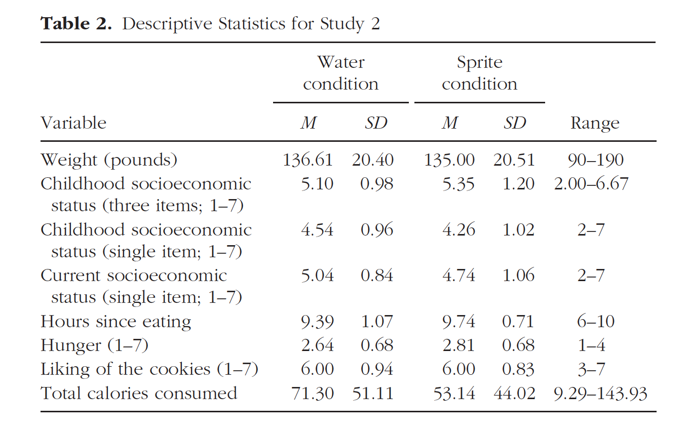
| Range | 42.690 - 396.505 |Study 2
The goal is to reproduce the values and formatting of this table.
knitr::include_graphics(here::here("img", "paper1_table2.png"))
Using arsenal
cleans2 <- cleans2 %>%
  mutate(condition = case_when(dummy2_sprite_water == 1 ~ "Water condition",
                               dummy1_water_sprite == 1 ~ "Sprite condition"
                               ))
table_two <- tableby(condition ~ weight_1 + child_ses + currnt_ses + hrs_no_eat_1 + hunglvl + delicious_taste + calories_eaten, data = cleans2)

my_labels <- list(
  weight_1 = "Weight (pounds)",
  child_ses = "Childhood socioeconomic status",
  currnt_ses = "Current socioeconomic status (single item; 1-7)",
  hrs_no_eat_1 = "Hours since eating",
  hunglvl = "Hunger (1-7)",
  delicious_taste = "Liking of the cookies (1-7)",
  calories_eaten = "Total calories consumed"
)
summary(table_two, labelTranslations = my_labels,
        title = "Table 2. Descriptive Statistics for Study 2")
| Sprite condition (N=31) | Water condition (N=29) | Total (N=60) | p value | |
|---|---|---|---|---|
| Weight (pounds) | 0.493 | |||
| Mean (SD) | 133.677 (19.666) | 137.241 (20.320) | 135.400 (19.896) | |
| Range | 90.000 - 180.000 | 107.000 - 190.000 | 90.000 - 190.000 | |
| Childhood socioeconomic status | 0.246 | |||
| Mean (SD) | 4.290 (0.973) | 4.586 (0.983) | 4.433 (0.981) | |
| Range | 2.000 - 6.000 | 2.000 - 7.000 | 2.000 - 7.000 | |
| Current socioeconomic status (single item; 1-7) | 0.247 | |||
| Mean (SD) | 4.774 (1.087) | 5.069 (0.842) | 4.917 (0.979) | |
| Range | 2.000 - 7.000 | 4.000 - 7.000 | 2.000 - 7.000 | |
| Hours since eating | 0.069 | |||
| Mean (SD) | 9.742 (0.682) | 9.207 (1.449) | 9.483 (1.142) | |
| Range | 7.000 - 10.000 | 4.000 - 10.000 | 4.000 - 10.000 | |
| Hunger (1-7) | 0.277 | |||
| Mean (SD) | 2.903 (0.790) | 2.690 (0.712) | 2.800 (0.755) | |
| Range | 2.000 - 5.000 | 1.000 - 4.000 | 1.000 - 5.000 | |
| Liking of the cookies (1-7) | 0.678 | |||
| Mean (SD) | 5.903 (0.870) | 6.000 (0.926) | 5.950 (0.891) | |
| Range | 4.000 - 7.000 | 3.000 - 7.000 | 3.000 - 7.000 | |
| Total calories consumed | 0.153 | |||
| Mean (SD) | 53.169 (44.756) | 70.924 (50.234) | 61.751 (47.918) | |
| Range | 9.286 - 139.287 | 13.929 - 143.930 | 9.286 - 143.930 |
Study 3
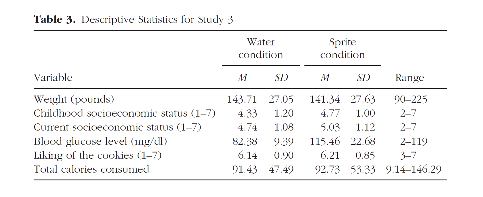
The goal is to reproduce the values and formatting of this table.
knitr::include_graphics(here::here("img", "paper1_table3.png"))
cleans3 <- cleans3 %>%
  mutate(condition = case_when(sprite_water_dummy2 == 1 ~ "Water condition",
                               water_sprite_dummy == 1 ~ "Sprite condition"
                               ))
table_three <- tableby(condition ~ weight + child_ses + adult_ses + blood_draw_2_post_maip + delicious_taste + calories_eaten, data = cleans3)

my_labels <- list(
  weight = "Weight (pounds)",
  child_ses = "Childhood socioeconomic status (1-7)",
  adult_ses = "Current socioeconomic status (1-7)",
  blood_draw_2_post_maip = "Blood glucose level (mg/dl)",
  delicious_taste = "Liking of the cookies (1-7)",
  calories_eaten = "Total calories consumed"
)
summary(table_three, labelTranslations = my_labels,
        title = "Table 3. Descriptive Statistics for Study 3")
| Sprite condition (N=41) | Water condition (N=42) | Total (N=83) | p value | |
|---|---|---|---|---|
| Weight (pounds) | 0.406 | |||
| Mean (SD) | 138.780 (26.729) | 143.714 (27.052) | 141.277 (26.843) | |
| Range | 103.000 - 196.000 | 95.000 - 225.000 | 95.000 - 225.000 | |
| Childhood socioeconomic status (1-7) | 0.192 | |||
| Mean (SD) | 4.659 (1.039) | 4.333 (1.203) | 4.494 (1.130) | |
| Range | 2.000 - 7.000 | 2.000 - 7.000 | 2.000 - 7.000 | |
| Current socioeconomic status (1-7) | 0.277 | |||
| Mean (SD) | 5.000 (1.095) | 4.738 (1.083) | 4.867 (1.091) | |
| Range | 3.000 - 7.000 | 3.000 - 7.000 | 3.000 - 7.000 | |
| Blood glucose level (mg/dl) | < 0.001 | |||
| Mean (SD) | 115.951 (21.561) | 82.381 (9.386) | 98.964 (23.579) | |
| Range | 73.000 - 183.000 | 62.000 - 119.000 | 62.000 - 183.000 | |
| Liking of the cookies (1-7) | 0.970 | |||
| N-Miss | 1 | 0 | 1 | |
| Mean (SD) | 6.150 (0.802) | 6.143 (0.899) | 6.146 (0.848) | |
| Range | 4.000 - 7.000 | 3.000 - 7.000 | 3.000 - 7.000 | |
| Total calories consumed | 0.935 | |||
| Mean (SD) | 92.321 (51.194) | 91.429 (47.486) | 91.869 (49.052) | |
| Range | 9.143 - 146.286 | 13.714 - 146.286 | 9.143 - 146.286 |
Using arsenal
table_three <- tableby(sprite_water_dummy2 ~ weight + child_ses + adult_ses + blood_draw_2_post_maip + delicious_taste + calories_eaten, data = cleans3)

my_labels <- list(
  weight = "Weight (pounds)",
  child_ses = "Childhood socioeconomic status (1-7)",
  adult_ses = "Current socioeconomic status (1-7)",
  blood_draw_2_post_maip = "Blood glucose level (mg/dl)",
  delicious_taste = "Liking of the cookies (1-7)",
  calories_eaten = "Total calories consumed"
)
summary(table_three, labelTranslations = my_labels,
        title = "Table 3. Descriptive Statistics for Study 3")
| 0 (N=41) | 1 (N=42) | Total (N=83) | p value | |
|---|---|---|---|---|
| Weight (pounds) | 0.406 | |||
| Mean (SD) | 138.780 (26.729) | 143.714 (27.052) | 141.277 (26.843) | |
| Range | 103.000 - 196.000 | 95.000 - 225.000 | 95.000 - 225.000 | |
| Childhood socioeconomic status (1-7) | 0.192 | |||
| Mean (SD) | 4.659 (1.039) | 4.333 (1.203) | 4.494 (1.130) | |
| Range | 2.000 - 7.000 | 2.000 - 7.000 | 2.000 - 7.000 | |
| Current socioeconomic status (1-7) | 0.277 | |||
| Mean (SD) | 5.000 (1.095) | 4.738 (1.083) | 4.867 (1.091) | |
| Range | 3.000 - 7.000 | 3.000 - 7.000 | 3.000 - 7.000 | |
| Blood glucose level (mg/dl) | < 0.001 | |||
| Mean (SD) | 115.951 (21.561) | 82.381 (9.386) | 98.964 (23.579) | |
| Range | 73.000 - 183.000 | 62.000 - 119.000 | 62.000 - 183.000 | |
| Liking of the cookies (1-7) | 0.970 | |||
| N-Miss | 1 | 0 | 1 | |
| Mean (SD) | 6.150 (0.802) | 6.143 (0.899) | 6.146 (0.848) | |
| Range | 4.000 - 7.000 | 3.000 - 7.000 | 3.000 - 7.000 | |
| Total calories consumed | 0.935 | |||
| Mean (SD) | 92.321 (51.194) | 91.429 (47.486) | 91.869 (49.052) | |
| Range | 9.143 - 146.286 | 13.714 - 146.286 | 9.143 - 146.286 |